DSP - Lab 2: 语谱图
本实验中,我们利用之前实现的 FFT 算法,生成了不同语音片段在不同窗口宽度下的语谱图。
Digital Signal Processing @ Fudan University, fall 2021.
实验简介
- 语音录制:三个单词发音 one, two, six;建议用 8 kHz 采样。
- 代码编写:要求使用你自己编写的 FFT 代码,不能调研已有函数库。
- 运行结果:(1) 画出语音波形图;(2) 画出不同窗口宽度(5 ms, 10 ms, 15 ms)的语谱图。
实验报告
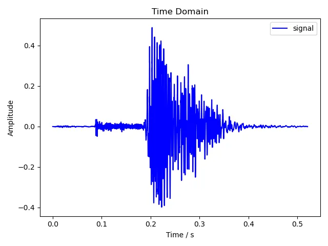
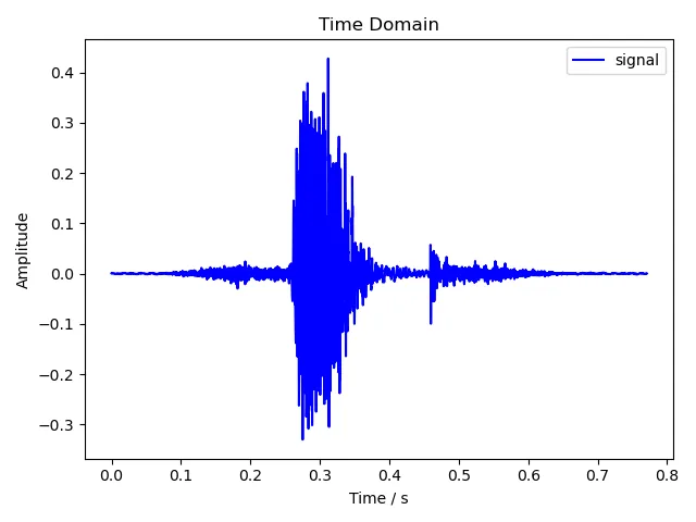
1 语音波形图
# main.py
def plot_waveform(filename: str, y: np.ndarray, sr: int) -> None:
'''
Plot the waveform of the audio signal.
Args:
`filename`: filename of the output figure
`y`: time series of the audio signal
`sr`: sample rate of the audio signal
'''
fig_time_path = fig_path / filename
n_samples = y.shape[0]
t = np.arange(n_samples) / sr
utils.plot_time_domain(fig_time_path, t, y)
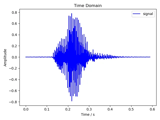
print(f'Output figure to "{fig_time_path}".')载入音频的过程就不再赘述了。这里绘制语音波形图的原理和上次绘制时域下的幅度图基本完全相同,区别是上次截取了前 1024 个采样,这次处理的则是整段音频。
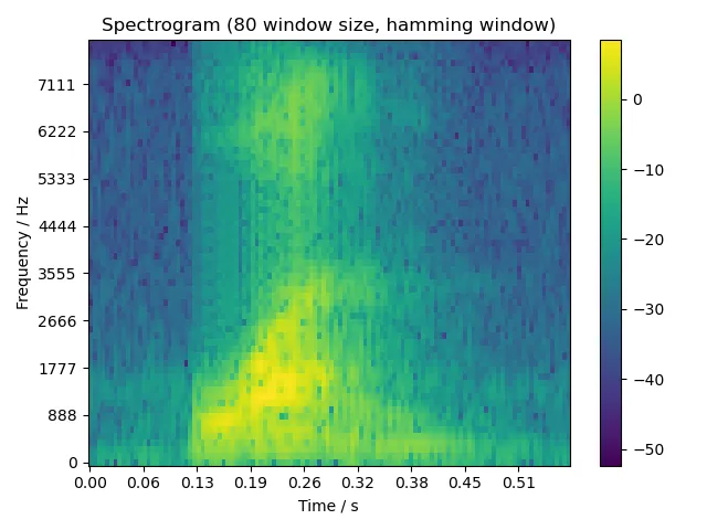
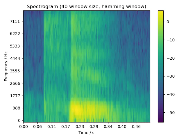
2 语谱图生成
生成语谱图的基本思想是使用 STFT(Short-time Fourier Transform)。由于直接对整段音频进行 FFT 的话,只能得到信号整体在频域下的幅度谱(只提供了有哪些频率成分的信息),而无法观察信号随时间变化的瞬时频率情况,因此我们就需要 STFT。STFT 采用滑动窗口的方式,随时间将此时的信号抽出一帧进行 FFT,如此即可得到信号的时间信息。
对于整段音频,我们预设一帧的窗口宽度,每次对这个窗口内的信号进行 FFT,将结果保存下来,然后将窗口向后滑动一段距离。这里窗口滑动的距离小于一个窗口宽度,从而确保与原来的窗口存在一定重叠,是为了尽量减少在边缘处由于窗口函数值趋近于零所导致的信息损失。通过不断滑动窗口逐帧进行 FFT,最后我们就得到了完整的语谱图。
# main.py

def create_spectrogram(y: np.ndarray, n_window: int) -> Tuple[np.ndarray, np.ndarray]:
    '''
    Create the spectrogram of the audio signal.

    Args:
        `y`: time series of the audio signal
        `n_window`: the number of samples used in each window

    Returns:
        `i_starts`: the starting indices of each window
        `spec`: the spectrum of frequencies of the audio signal as it varies with time
    '''

    n_samples = y.shape[0]
    i_starts = np.arange(0, n_samples, n_window // 2, dtype=int)
    i_starts = i_starts[i_starts + n_window < n_samples]
    n_fft = utils.next_pow2(n_window)
    zero_padding = np.zeros(n_fft - n_window)
    spec = np.array([np.abs(fft(
        np.concatenate((hamming(n_window) * y[i:i+n_window], zero_padding))
    )[:n_fft // 2]) for i in i_starts])
    # Rescale the absolute value of the spectrogram.
    spec = 10 * np.log10(spec.T + np.finfo(float).eps)
    return i_starts, spec
此处 i_starts 即每个窗口的开始位置(采样的索引),每次窗口向后滑动的距离为半个窗口宽度,直到剩余信号长度不足一个窗口宽度为止。这里由于我们自行实现的 FFT 算法仅支持处理 2 的幂的信号长度,因此对需要处理的信号进行了补零操作。
spec = np.array([np.abs(fft(
    np.concatenate((hamming(n_window) * y[i:i+n_window], zero_padding))
)[:n_fft // 2]) for i in i_starts])
这段看起来有点复杂,其实就是根据 i_starts 中的开始位置遍历整段信号 y,每次取一帧信号 y[i:i+n_window],加汉明窗 hamming(n_window),然后补零。之后就和上次分析信号在频域下的幅度谱时一样了,对信号进行 FFT,取模。这里直接取了 FFT 结果的前一半,是因为原始信号是实数信号,其 FFT 结果是对称的。最后将所有帧的 FFT 结果组成一个矩阵,就是我们需要的语谱图了。
此处汉明窗的函数式为:
$$w(n) = 0.54 - 0.46\cos(\frac{2\pi n}{M-1})\qquad (0\le n\le M-1)$$
其实现如下:
# windows.py

def hamming(m: int) -> np.ndarray:
    '''
    Return the Hamming window.

    Args:
        `m`: number of points in the output window

    Returns:
        The Hamming window of size `m`.
    '''

    if m < 1:
        return np.array([])
    if m == 1:
        return np.ones(1)
    n = np.arange(m)
    return 0.54 - 0.46 * np.cos(2 * np.pi * n / (m - 1))
最后我们将此矩阵转置,并将信号幅度的计量单位转换为 dB。
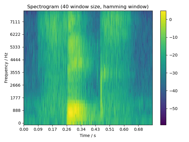
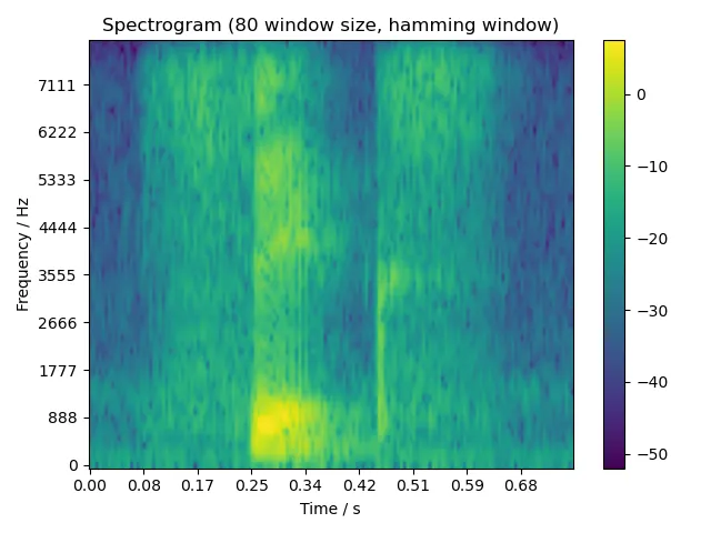
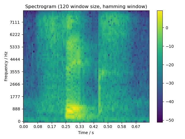
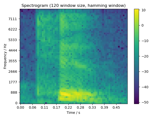
由于题目要求窗口宽度为 5 ms, 10 ms, 15 ms,考虑到我们音频的采样率为 8000 Hz,因此调用本函数时,相应的窗口宽度即为 40, 80, 120 个采样。
3 语谱图绘制
生成完语谱图后,我们将其绘制出来。
# main.py

fig_path = Path('assets/spectrogram/dev_set')

def plot_spectrogram(
    filename: str, i_starts: np.ndarray, spec: np.ndarray, sr: int
) -> None:
    '''
    Plot the spectrogram of the audio signal.

    Args:
        `filename`: filename of the output figure
        `i_starts`: the starting indices of each window
        `spec`: the spectrogram to plot
        `sr`: sample rate
    '''

    fig_spec_path = fig_path / filename
    xticks = np.linspace(0, spec.shape[1], 10)
    xlabels = [f'{i:4.2f}' for i in np.linspace(0, i_starts[-1] / sr, 10)]
    yticks = np.linspace(0, spec.shape[0], 10)
    ylabels = np.floor(fft_freq(spec.shape[0], sr, yticks)).astype(int)
    utils.plot_spectrogram(
        fig_spec_path, spec, xticks, xlabels, yticks, ylabels, n_window,
    )
    print(f'Output figure to "{fig_spec_path}".')
这里主要是要将 x 轴和 y 轴恢复成正确的时间和频率单位。目前 x 轴上的值是采样的索引,因此将其除以采样率 sr,就得到正确的时间了。y 轴上的值则需要通过函数 fft_freq() 从 FFT 结果转换为表示的频率,其实现就是乘上采样率 sr 再除以 FFT 处理的信号长度 n_fft,这里可以通过 FFT 结果的长度 spec.shape[0] 得到。
此处为了显示上的美观,x 轴和 y 轴各取 10 个刻度。
最后就是调用 matplotlib.pyplot 库的 API 进行绘制了。
# utils.py

def plot_spectrogram(
    output_path,
    spec: np.ndarray,
    xticks: np.ndarray,
    xlabels: np.ndarray,
    yticks: np.ndarray,
    ylabels: np.ndarray,
    n_fft: int,
) -> None:
    '''
    Plot the spectrogram of a wave.

    Args:
        `output_path`: path to the output figure
        `spec`: the spectrogram to plot
        `xticks`: tick locations of the x-axis
        `xlabels`: tick labels of the x-axis
        `yticks`: tick locations of the y-axis
        `ylabels`: tick labels of the y-axis
        `n_fft`: the number of samples for the FFT
    '''

    plt.figure()
    plt.title(f'Spectrogram ({n_fft} window size, hamming window)')
    plt.xticks(xticks, xlabels)
    plt.xlabel('Time / s')
    plt.yticks(yticks, ylabels)
    plt.ylabel('Frequency / Hz')
    plt.imshow(spec, origin='lower', aspect='auto')
    plt.colorbar(use_gridspec=True)
    plt.tight_layout()
    plt.savefig(output_path)
4 运行代码
4.1 安装
配置环境前,首先需要安装以下依赖:
- Anaconda 2022.05 或以上(含 Python 3.9)
然后创建并激活 conda 虚拟环境,同时安装所有依赖包:
conda env update --name dsp --file environment.yml
conda activate dsp
4.2 使用
将音频文件放置于 ./data/dev_set 目录下,执行以下命令启动程序:
python3 main.py生成的语音波形图和语谱图将保存在 ./assets/spectrogram 目录下。
4.3 测试
本实验中,我们使用了预录制的音频文件 one.dat, two.dat, six.dat,其内容分别是单词 one, two, six 的单词发音,按 8000 Hz 采样。如果你的测试音频不是按 8000 Hz 采样的,可以使用 resample.py 进行重采样,使用方法:
python3 resample.py "path/to/foobar.wav" 8000  # 单个文件
python3 resample.py "path/to/directory" 8000    # 目录下所有 .wav 文件递归批处理
重采样后的音频文件将保存在同目录下,文件名的后缀名修改为 .dat。
运行程序后,程序将在 ./assets/spectrogram 目录下生成以下文件:
foobar_time_domain.png:原音频foobar.dat的语音波形图foobar_spec_domain_5ms_hamming.png:信号在 5 ms 窗口宽度下的语谱图foobar_spec_domain_10ms_hamming.png:信号在 10 ms 窗口宽度下的语谱图foobar_spec_domain_15ms_hamming.png:信号在 15 ms 窗口宽度下的语谱图
5 运行结果
5.1 语音波形图
5.1.1 one
5.1.2 two
5.1.3 six
5.2 语谱图
5.2.1 one


5.2.2 two

5.2.3 six